
Simulations
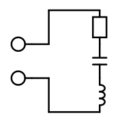
In the last chapter we discussed an RLC circuit. We solved the differential equation system and plotted the result using the 2D graph feature of Cassiopeia. In this chapter we want to show how to handle problems that cannot be solved analytically and therefore must be simulated. Consider the following circuit and assume that a square wave with some duty cycle is applied to the leads.
 |
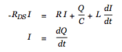
We handle the pulse on case first. Pulse on means we have
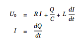 |
 |
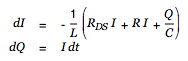
for the second equation. The first equation can be rewritten as follows:
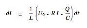 |
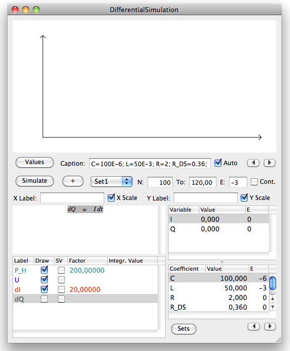
More preparation is not needed to simulate the circuit shown above. Choose SDM - Simulation from the Cassiopeia menu. The simulation inspector appears. Drag the two differential equations we have just derived onto the textview of the simulation inspector.
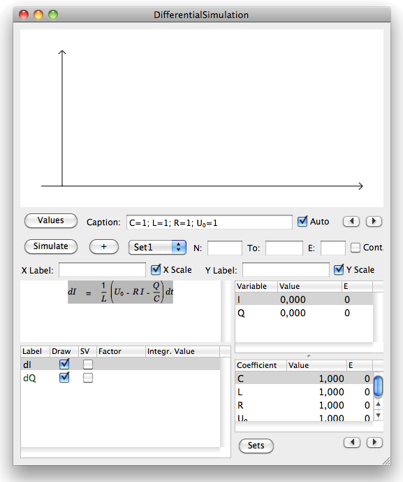 |
Specify reasonable values for the referenced coefficients and check/set the start values for the two variables I and Q. You might also want to open Tools - Colors and drag colors onto the two differential expressions in the tableview.
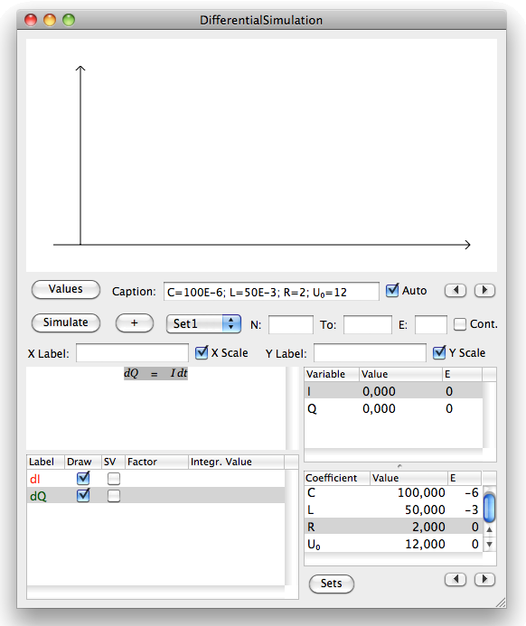 |
The final step before running the first simulation is specifying the time frame and the number of simulation steps. We specify 100 steps in the N: field and 100ms in the To: and E: field and then click on Simulate.
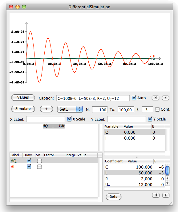 |
The wave form for the current looks reasonable. The wave form for the charge is of less interest. We probably would rather like to present the voltage in the cap instead. The relation between charge and voltage is given by
We simply drag this equation onto the textview in the simulation inspector, assign a label and a color and rerun the simulation by clicking on Simulate again.
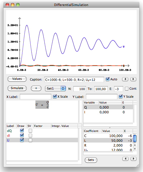 |
The current needs a scaler now. We uncheck the draw field for the charge to suppress it being drawn.
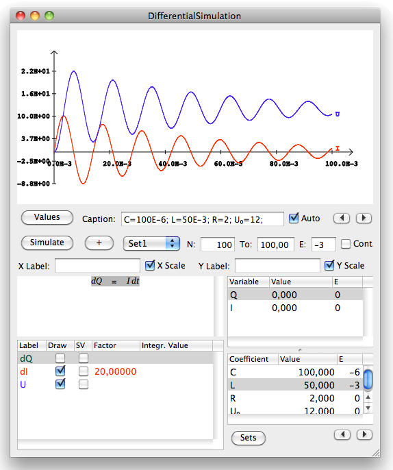 |
Let's assume we are interested in the heat loss due to the resistance in the circuit. The heat loss is given by
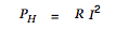 |
We simply drag this equation onto the textview on the simulation inspector, set a reasonable scaler and a color and rerun the simulation.
 |
So far we have discussed the pulse on phase only and simulated the circuit over the first 100ms. However, our original intent was to a apply a square wave to the input. We need to discuss the pulse off phase now. A perfect short of the leads is unrealistic. We therefore assume that the input leads are shorted with a switched on MOSFET with a small but greater than zero resistance. This gives us the following set of differential equations for the off phase.
 |
These equations need to be rewritten as differential expressions again.
 |
We are done with the math. (Re)open the simulation inspector and note the Sets button below the coefficient tableview. Click on this button to open the set inspector.
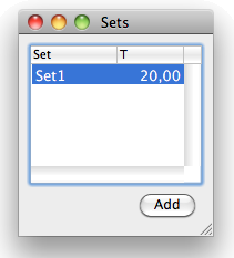 |
A default set named Set1 was created automatically when the simulation was added to our document. We were working with this default set so far. Click on the Add button to create a second set for the pulse off phase. Name it Set2 and set its duration to 20ms as well.
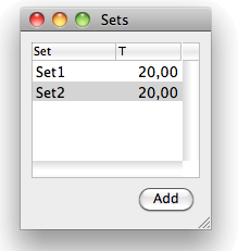 |
Close the set panel and get back to the simulation inspector. Note that we can switch back and forth between Set1 and Set2 using the popup button in the middle of the inspector. No equations have been attached to the second set so far.
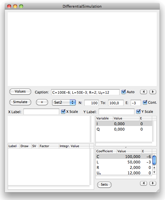 |
Drag the two differential expressions for the off phase onto the textview. Then drag the equations for the heat loss and the voltage onto the textview as well to complete the equation set for the off phase. Set the same scalers and the same colors.
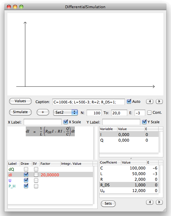 |
The off phase (MOSFET on) resistance was set to 1 per default. We set a more realistic value of 0.36 in the coefficient tableview. Moreover we set the total simulation time to 120ms. This gives us three on and off pulses.
 |
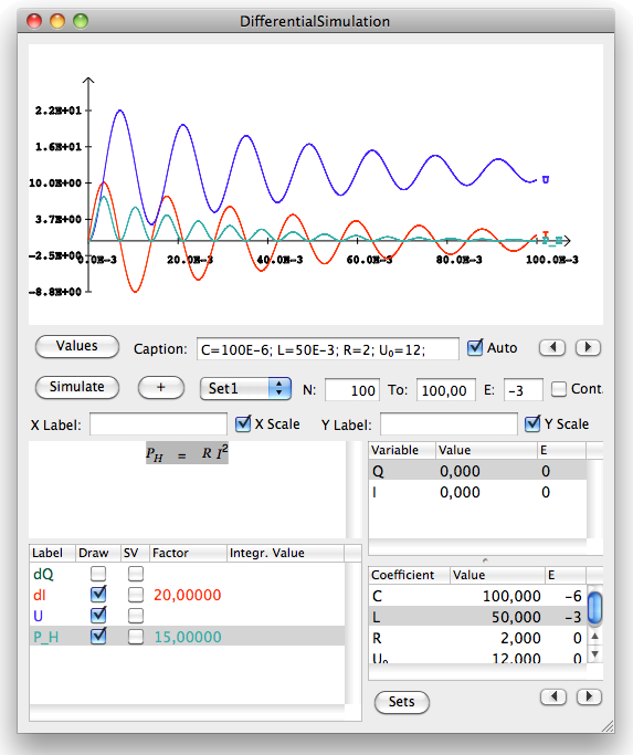
Click on Simulate now to run the simulation.
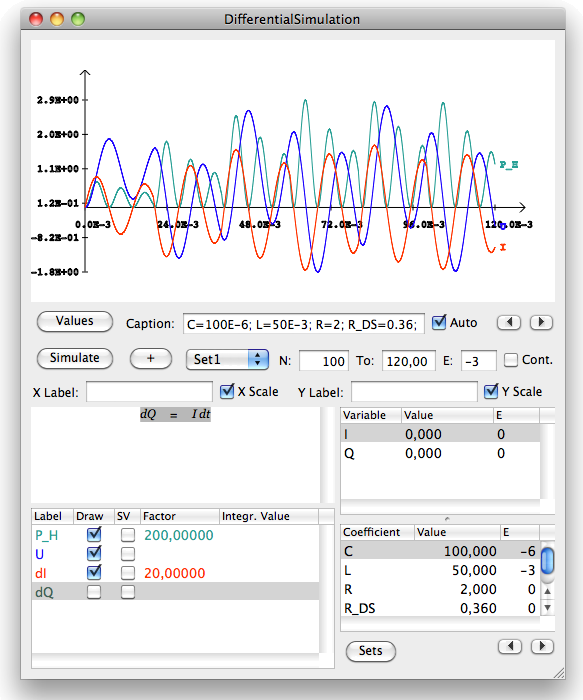 |
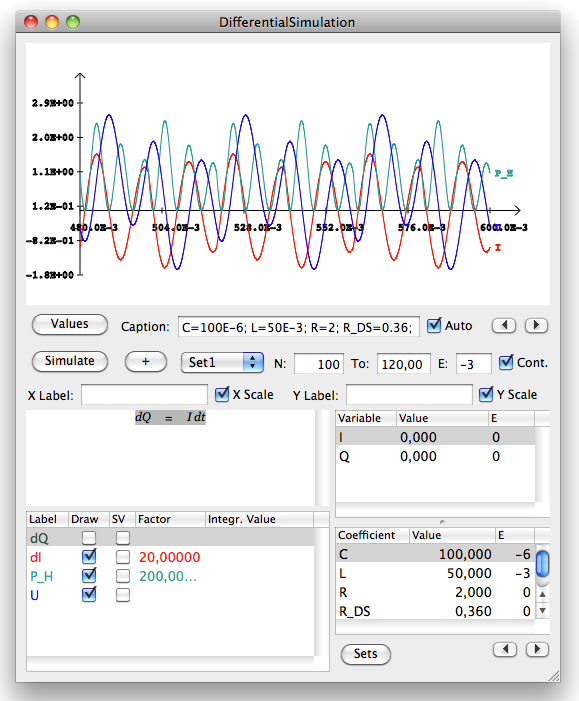
This gives us the behaviour of the circuit in the first 120ms. Check the Cont. box and run the simulation again. This extends the simulation time by a factor of five and allows us to examine the long term development of the circuit properties. The two little arrows next to the caption auto checkbox can be used to navigate through the simulation result.
 |
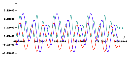
Clicking into the document populates the graph into your text.
 |
News
| 05.04.2013 | Cassiopeia 1.1.9 released |
| 04.04.2013 | Links and Bibliography |
| 01.04.2013 | Books |
| 30.03.2013 | Documents |
| 28.03.2013 | Simulations |
| 22.03.2013 | Introductory Pricing until April 30, 2013 |
| 16.03.2013 | 2D Graphs |
| 10.03.2013 | Symbolic Algebra |
| 08.03.2013 | Getting Started |
| 07.03.2013 | Installation and Setup |
Partner
· FrontBaseContact
Acrux GmbH Advanced Science SubdivisionSales: sales@advanced-science.com
Support: support@advanced-science.com
