
2D Graphs
Cassiopeia includes a sophisticated 2D graph module for plotting functions. We will discuss a damped LC tank in this document and then present the result of the derivation in a 2D graph. If you are not interested in the concrete physical problem skip the math and scroll down to the graphs. :-) We consider the following electrical circuit consisting of a capacitance, a resistor and an inductance.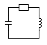 |
This circuit is described mathematically by the following two differential equations:
 | (1) |
 | (2) |
The first equation can be rewritten as follows:
 | |
 |
We use the following approach to solve this linear differential equation:
 | |
 | |
 |
 | |
 |
The last equation is true for all t only if we assume
 |
This gets us
 |
 | |
 | |
 | |
 |
We consider the first solution and insert the expression into our solution apporach.
 | |
 | |
 | |
 |
We set
 |
and use Euler to rewrite
 | |
 |
The differential equation is linear. Therefore both summands must be a solution for the differential equations.
 | |
 |
A constant factor shouldn't harm a solution and the sum of two solutions is again a solution. We can thererefore write
 |
This can be transformed to
 |
 |
We now use Eq. 2 to get an expression for the current in the circuit.
 |
 |
We Alt-drag the expression for the angular frequency onto this last equation and replace Q with CU. This gets us the following two functions.
 |
 |
Now choose SDM - FunctionGraph2D from the menu to insert a 2DGraph and drag the two equations onto the textview of the FunctionGraph2D inspector.
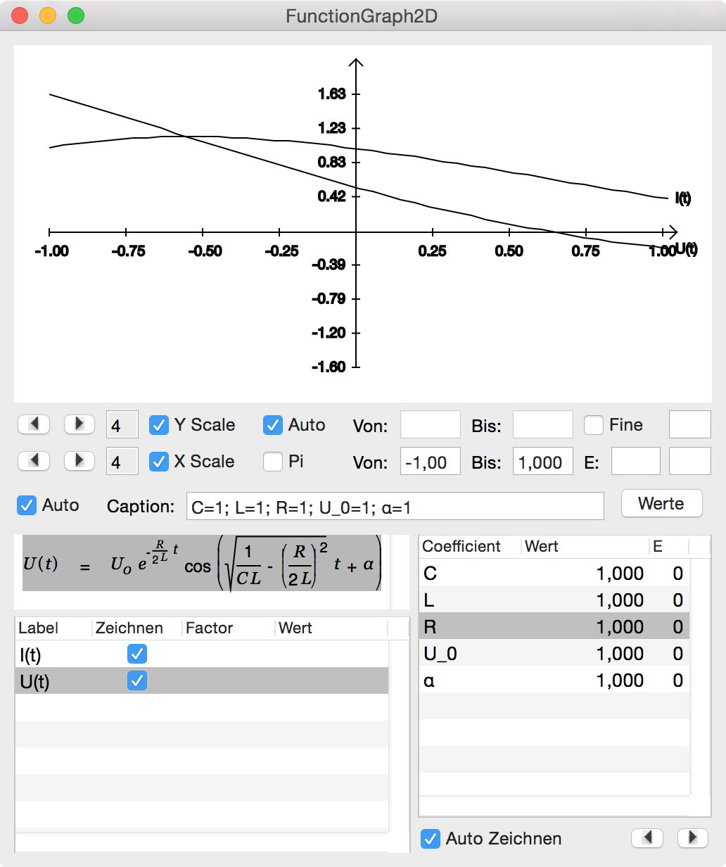 |
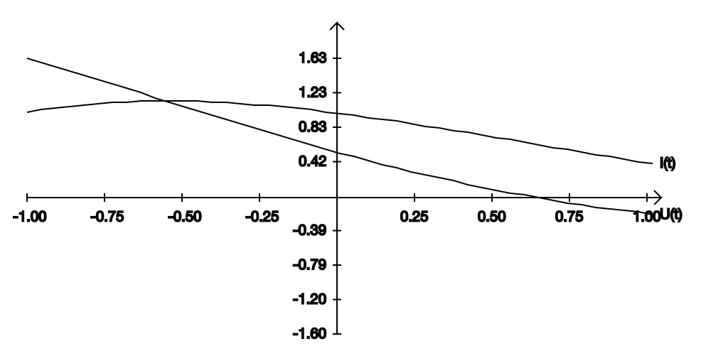
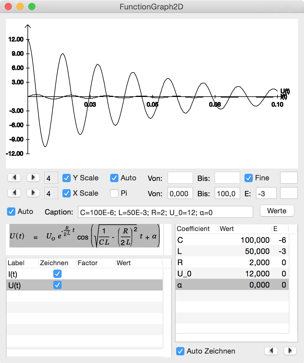
The graph appears as follows In our document.
 |
We change the From: and To: values for the abscissa to 0 - 100 ms. After modifying the values press <Return> in one of the fields to trigger redraw of the graph.
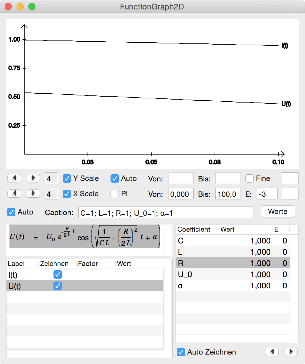 |
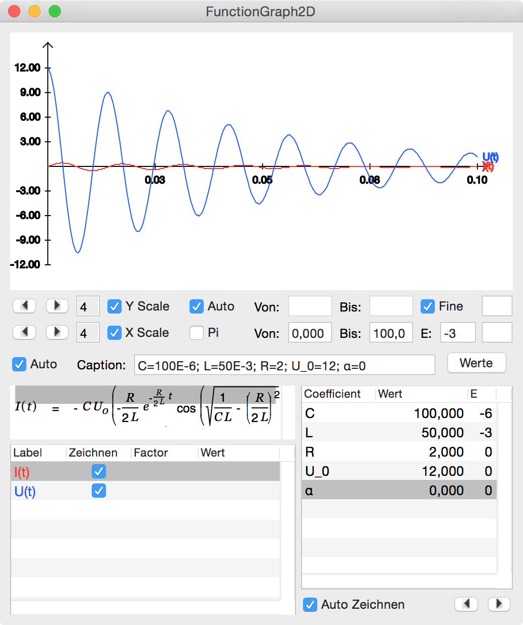
Now change the coefficients C, L and R to more realistic values. Also check the Fine box to get a more accurate rendering of the graph.
 |
Choose Tools - Colors from the menu and drag red color onto the current function in the tablevie win the lower left and blue color onto the function for the voltage.
 |
This does not look too bad. However, the current line is too flat to be easily examined. We therefore specify a scale factor of ten for the current function.
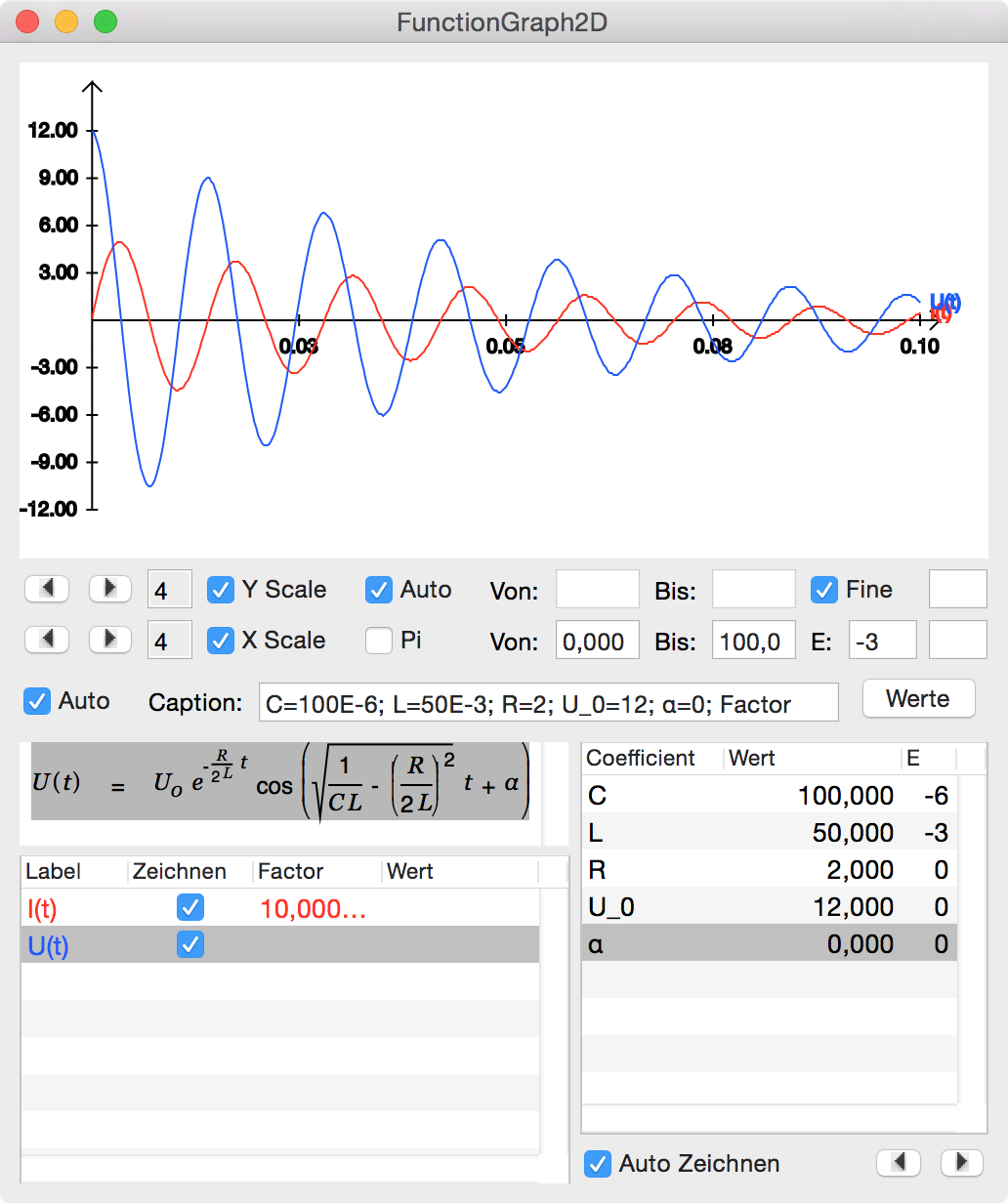 |
Click back into your document. The graph is updated accordingly.
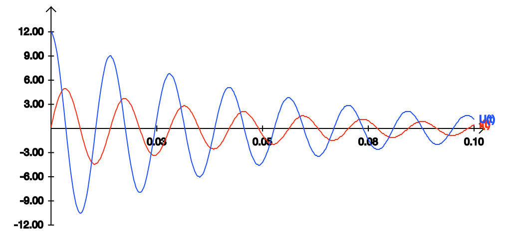 |
We are not done yet. Let's assume we are interested in the heat loss in the wire resistance. This loss is given by
 |
We Alt-drag the expression for the current onto this equation and get
 |
We now double-click onto the 2D graph to (re)open its inspector and simply drag this last equation onto the textview. We also drag the expression for
 onto the textview and set a scaler of 20 and a color for this additional physical property.
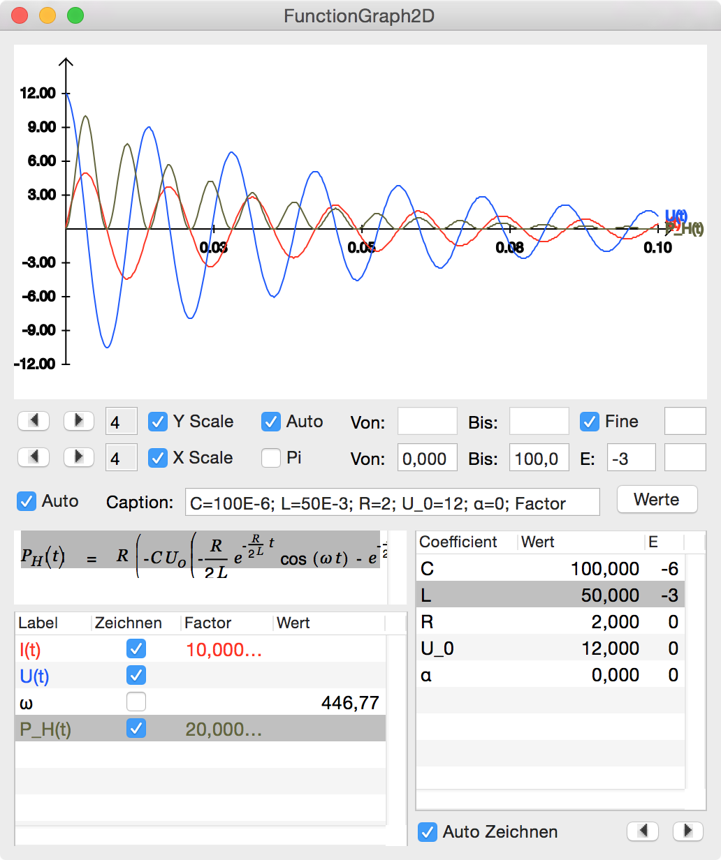 |
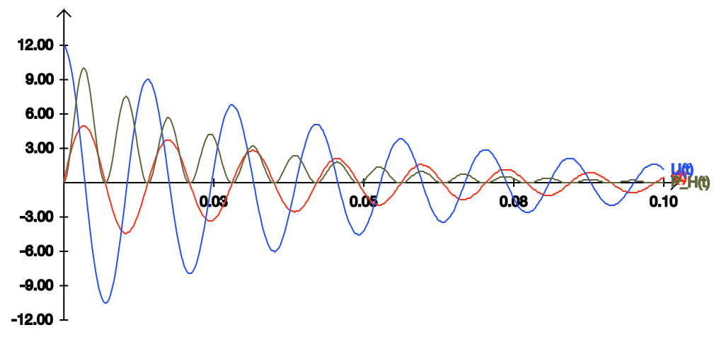
Clicking back into the document updates the 2D graph.
 |
The functions in a 2D graph can be interdependent. Assume the result of your creative work is the following set of functions (see Example Paper):
 | |
 | |
 | |
 | |
 |
Note that the last function depends on all the other. These functions can be dragged as they are onto a 2D graph to be plotted.
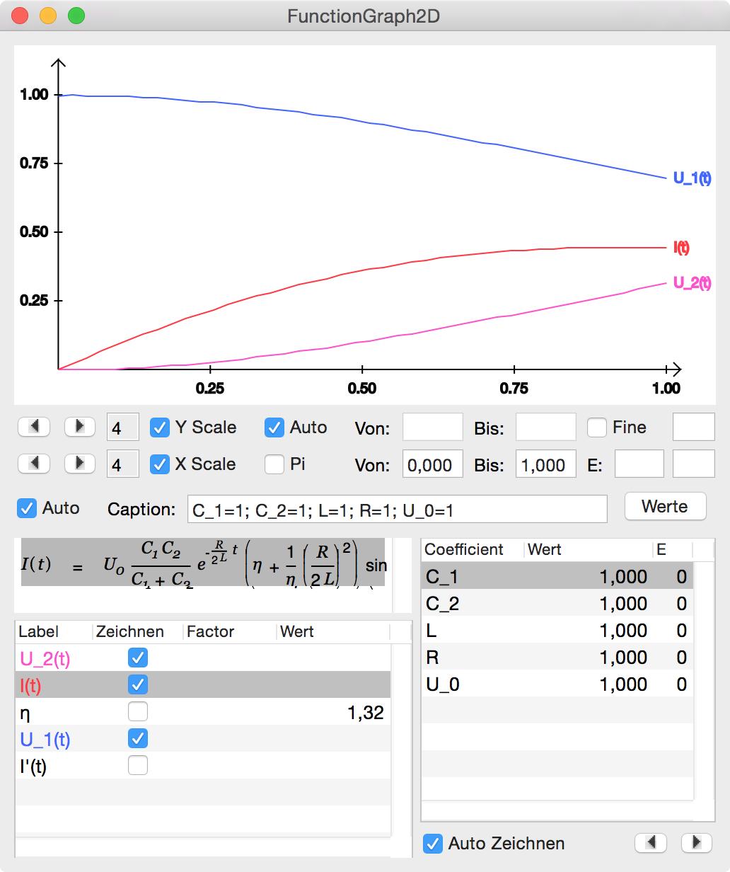 |
News
| 23.04.2023 | Cassiopeia 2.9.0 released |
| 05.10.2022 | Cassiopeia 2.8.3 released |
| 29.09.2022 | Cassiopeia 2.8.0 released |
| 08.07.2022 | Cassiopeia 2.7.0 released |
| 14.04.2021 | Cassiopeia 2.6.5 released |
| 10.02.2021 | Cassiopeia 2.6.1 released |
| 26.06.2015 | Word Processor Comparison |
| 24.06.2015 | Updated Documentation |
| 23.06.2015 | Cassiopeia Yahoo Group |
| 18.06.2015 | Advanced Data Security |
| 11.05.2015 | Cassiopeia Overview |
| 08.05.2015 | Exporting to files |
| 14.05.2013 | LaTeX and HTML Generation |
| 08.05.2013 | Example Paper released |
| 26.04.2013 | Co-editing in a workgroup |
| 16.04.2013 | Equation Editor Quick Reference |
| 12.04.2013 | Equation Editor |
| 04.04.2013 | Links and Bibliography |
| 01.04.2013 | Books |
| 30.03.2013 | Documents |
| 28.03.2013 | Simulations |
| 16.03.2013 | 2D Graphs |
| 10.03.2013 | Symbolic Algebra |
| 08.03.2013 | Getting Started |
| 07.03.2013 | Installation and Setup |
White Papers
| 13.10.2015 | 01 Writing documents |
| 15.10.2015 | 02 Using the equation editor |
Youtube
| 08.07.2022 | Installation & Getting Started |
| 14.04.2021 | Animating Wave Functions |
| 26.01.2016 | Keystroke Navigation |
| 22.10.2015 | Equation Editor Demo |
| 19.06.2015 | Equation Editor Tutorial |
| 10.06.2015 | Sections and Equations |
| 09.06.2015 | Getting Started |
| 09.06.2015 | Damped Oscillations |
| 29.05.2015 | Solving equations |
| 13.05.2015 | Privileges and Links |
| 19.06.2013 | Magnetic Field |
| 14.06.2013 | Creating Documents |
| 10.06.2013 | Vector Algebra |
| 30.05.2013 | Differential Simulations |
Contact
Smartsoft GmbH Advanced Science Subdiv.Support: support@advanced-science.com
