
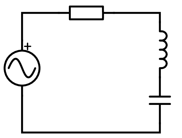
Damped LC tank with external excitation
We consider a resistor, an inductance and a cap in series excited by an external AC signal.
 |
This circuit is mathematically described by
 | |
 | |
 | (1) |
Solving the homogeneous part of the differential equation
We solve the homogeneous part of the differential equation Eq. 1 first
 | (2) |
 | |
 | |
 |
Substitution into the differential equation gives
 | |
 |
This equation is true for all
 only if
 |
is true. We solve this as follows:
 | |
 |
 | |
 |
 | |
 | |
 |
We define
 |
 | |
 | |
 | |
 |
 | |
 | |
 | |
 |
The general solution for the homogeneous differential equation can therefore be written as
 | |
 | |
 | |
 |
or after replacing the factors
 |
Since the differential equation is linear we can rewrite this as follows
 |
or even shorter like so
 | (3) |
 | (4) |
 | (5) |
 | (6) |
with the two freely choosable constants
 und
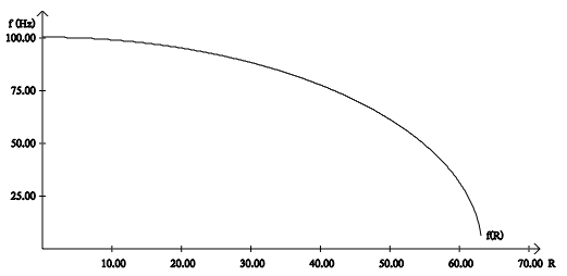
und  . Please note the dependence of the resonance frequency from the resistance.
 | (7) |
 |
Finding a particular solution for the inhomogeneous differential equation
We find a particular solution for the inhomogeneous differential equation by trying a suitable approach.
 |
A suitable approach for the above equation is
 | |
 | |
 |
Substituted into the differential equation we get
 | |
 | |
 | |
 |
 | |
 | |
 | |
 |
The value
 is the length of the complex number on the right.
 | |
 |
The angle
 is determined as follows:
 | |
 | |
 |
 | |
 | |
 |
 | |
 | |
 |
 |
Combining the general and the particular solution
We combine the general solution for the homogeneous differential equation
 | |
 | |
 | |
 |
and the particular solution of the inhomogeneous differential equation
 | |
 | |
 |
into a total solution by summation:
 | (8) |
Since the e-Function approaches 0 for large values of
 only the particular solution remains after an initiation period.
 | (9) |
We devide by
 to get the voltage in the cap, take first derivatives to get the current and take the second derivative to get the voltage over the coil.
 | |
 | |
 | |
 | |
 | |
 | |
 |
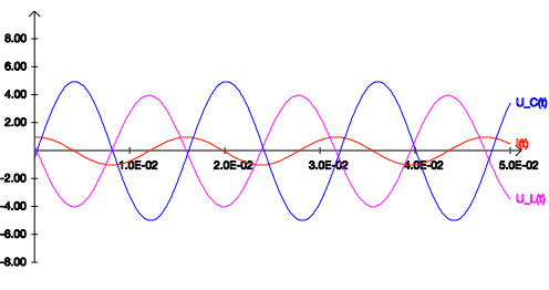 |
We determine the peak voltage in the cap and the peak current with respect to
 (resonance frequency):
 | |
 | |
 | |
 |
 | |
 | |
 | |
 |
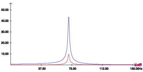 |
If we excite the series tank with its resonance frequency we get high voltages over the components and a very high current only limited by the resistance of the wire.
Energy Consideration
The power going into the circuit is given by | |
 | |
 | |
 | |
 | |
 | |
 | |
 |
 |
This gets us the following expression for the input power.
 | (10) |
 | |
 |
The circulating power in the circuit is defined as
 |
with
 |
 | |
 |
 | |
 | |
 | |
 | |
 | |
 | |
 | |
 | |
 | |
 | |
 | |
 | |
 |
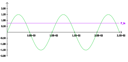 |
We have scaled
 with a factor of 100 in the figure above. The Input power is very small compared to the circulating power for
  .
.News
| 23.04.2023 | Cassiopeia 2.9.0 released |
| 05.10.2022 | Cassiopeia 2.8.3 released |
| 29.09.2022 | Cassiopeia 2.8.0 released |
| 08.07.2022 | Cassiopeia 2.7.0 released |
| 14.04.2021 | Cassiopeia 2.6.5 released |
| 10.02.2021 | Cassiopeia 2.6.1 released |
| 26.06.2015 | Word Processor Comparison |
| 24.06.2015 | Updated Documentation |
| 23.06.2015 | Cassiopeia Yahoo Group |
| 18.06.2015 | Advanced Data Security |
| 11.05.2015 | Cassiopeia Overview |
| 08.05.2015 | Exporting to files |
| 14.05.2013 | LaTeX and HTML Generation |
| 08.05.2013 | Example Paper released |
| 26.04.2013 | Co-editing in a workgroup |
| 16.04.2013 | Equation Editor Quick Reference |
| 12.04.2013 | Equation Editor |
| 04.04.2013 | Links and Bibliography |
| 01.04.2013 | Books |
| 30.03.2013 | Documents |
| 28.03.2013 | Simulations |
| 16.03.2013 | 2D Graphs |
| 10.03.2013 | Symbolic Algebra |
| 08.03.2013 | Getting Started |
| 07.03.2013 | Installation and Setup |
White Papers
| 13.10.2015 | 01 Writing documents |
| 15.10.2015 | 02 Using the equation editor |
Youtube
| 08.07.2022 | Installation & Getting Started |
| 14.04.2021 | Animating Wave Functions |
| 26.01.2016 | Keystroke Navigation |
| 22.10.2015 | Equation Editor Demo |
| 19.06.2015 | Equation Editor Tutorial |
| 10.06.2015 | Sections and Equations |
| 09.06.2015 | Getting Started |
| 09.06.2015 | Damped Oscillations |
| 29.05.2015 | Solving equations |
| 13.05.2015 | Privileges and Links |
| 19.06.2013 | Magnetic Field |
| 14.06.2013 | Creating Documents |
| 10.06.2013 | Vector Algebra |
| 30.05.2013 | Differential Simulations |
Contact
Smartsoft GmbH Advanced Science Subdiv.Support: support@advanced-science.com
